Neural ODE and Optimal Control

Reference. Prof. Li Qianxiao’s lecture notes on optimal control.

Links to the materials: GitHub repository.

Formulation of Optimal Control Problems

Consider the ODE $\dot{x}(t) = f(t, x(t), u(t))$ for $t \in [t_0, t_1]$, with $x(t_0) = x_0$.

The Bolza problem with a Lagrangian $L(t, x(t), u(t))$ and a terminal cost function $\Phi(t_1, x(t_1))$ is stated below

Pontryagin’s Maximum Principle

By the Pontryagin’s maximum principle (PMP), the optimal control $u^\ast$ and the corresponding state trajectory $x^\ast$ and co-state trajectory $p^\ast$ must satisfy

where the Hamiltonian $H(t,x, p, u) = p^\top f(t, x, u) - L(t, x, u)$.

The method of successive approximations (MSA) is based on the PMP.

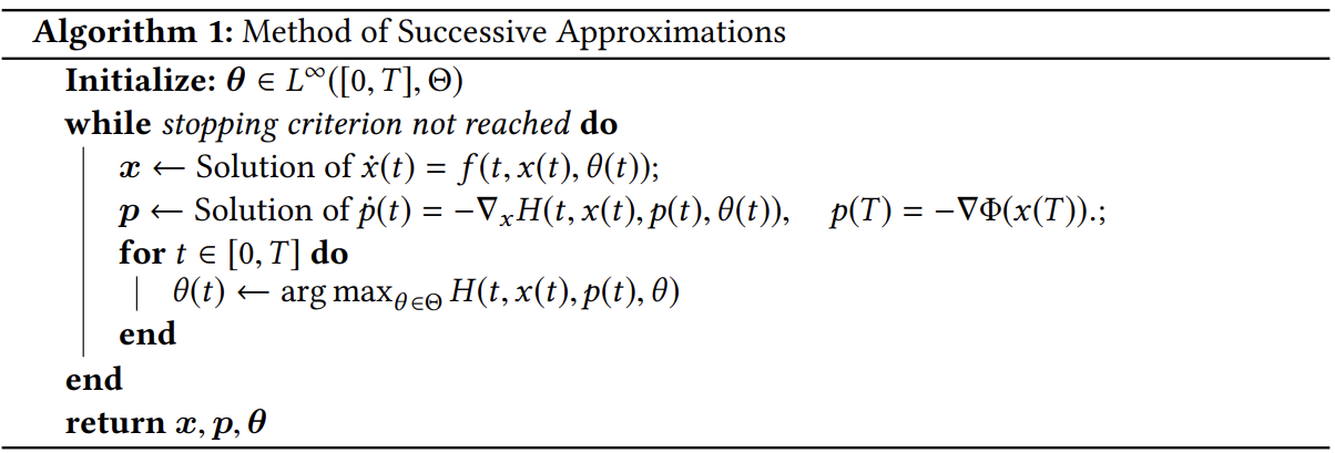
Remark. We use $u(\cdot)$ to denote the control instead of $\theta(\cdot)$ as in the above algorithm. We will use $u(\cdot)$ unless otherwise mentioned.

Moreover, the update step \[ u(t) \gets \text{argmax}_u H(t, x(t), p(t), u) \] could be replaced by some gradient update rule \[ u_t \gets u_t + \eta \cdot \nabla_u H(t, x_t, p_t, u_t) \] according to the following improvement guarantee (subject to some mild assumptions)

where $x_t$ and $p_t$ are computed from $u$, and $S[u] = \int_{t_0}^{t_1} H(t, x_t, p_t, u^\prime)\,dt$. Thus, a sufficiently small perturbation that increases the integrated Hamiltonian yields an improved control.

Neural ODE

We attempt to interpret the adjoint sensitivities algorithm used in Neural ODEs in the context of optimal control. In particular, consider the Mayer problem for simplicity

Assume that the control $u_\theta(\cdot)$ is parameterized by $\theta \in \Theta$ (for example, by an MLP). We can then reformulate the original problem as

where $\theta(t) \equiv \theta$ is a constant and $g(t, x(t), \theta(t)) = f(t, x(t), u_\theta(t))$. By the adjoint sensitivities algorithm, the following gradient update rule with learning rate $\eta$ should be applied

where

with $H(t, x, p, \theta) = p^\top g(t, x, \theta)$. We may observe that this is equivalent to a variant of the MSA using the steepest ascent.

By the PMP, the optimal parameter $\theta^\ast$ satisfies

Notice that the last condition necessarily requires

Some intuitions behind our focus on this relaxed condition could be:

1. From the improvement guarantee aforementioned, we only need to locally optimize the integral of the Hamiltonian;

2. Assuming we are using the MSA to solve this converted problem, since we want the neural network parameters to be a constant, we could average the updated parameters at different timesteps, which results in an integral.

Consequently, it makes sense to use the following gradient update rule with learning rate $\eta$

Interchanging integration and differentiation shows that this is equivalent to the adjoint-sensitivity update for a Mayer problem. A Bolza problem adds a nonzero running cost, which can be interpreted as a regularization term.

Hamilton-Jacobi-Bellman Equation

The PMP is a necessary condition for optimal control, a sufficient condition could be the Hamilton-Jacobi-Bellman (HJB) equations. It is similar to the Bellman equations in the context of reinforcement learning. Firstly, we need to define the value function

The value function $V(s,z)$ is the minimum cost attainable from state $z$ at time $s$.

The HJB equation is given by \[ \partial_t V(t, x) + \inf_{u}{L(t, x, u) + [\nabla_x V(t, x)]^\top f(t, x, u)} \quad \text{ s.t. } \quad V(t_1, x) = \Phi(x). \] The PMP and HJB formulations are closely related. Along an optimal trajectory, the co-state can be identified with $p=-\nabla_x V(t,x)$; this is the adjoint appearing in the Neural ODE paper under the sign convention used here.

Linear Quadratic Regulator (LQR)

Consider the following controlled linear dynamical system \[ \dot{x}_t = A(t)x_t + B(t)u_t \qquad A(t) \in \mathbb{R}^{d\times d}, \quad B(t) \in \mathbb{R}^{d \times m}, \quad u_t \in \mathbb{R}^m, \quad t \in [0, T] \] with the cost functional \[ J[u] = x_T^\top M x_T + \int_0^T x_t^\top Q(t) x_t + u_t^\top R(t) u_t dt \] where $M\in\mathbb{R}^{d\times d}$ is symmetric positive semidefinite and $Q(t)$ and $R(t)$ are symmetric positive definite.

The quadratic value function $V(t,x)=x^\top P(t)x$ satisfies the HJB equation when $P(t)$ solves the following Riccati differential equation: \[ \dot{P}(t) = -P(t)A(t)-A^\top(t)P(t)-Q(t)+P(t)B(t)R^{-1}(t)B^\top(t)P(t), \quad P(T)=M. \] satisfies the HJB equations for the LQR problem. Furthermore, the optimal control $u^\ast$ could be extracted by \[ u^\ast(t) = -R^{-1}(t)B^\top(t)P(t)x^\ast(t). \] This provides a baseline obtained by numerically solving the RDE.

A Simple Application

Consider the following controlled system (say, of a vehicle)

where $\alpha(t)$ is the resistance at time $t$. Starting from $(x_0,v_0)=(1,0)$, we seek to bring $x_1$ close to the origin while penalizing control effort by $\lambda u_t^2$. This gives the optimal-control problem

We could solve this LQR problem based on the RDE method (which should be more reliable in this simple problem) and the Neural ODE. The results are plotted below

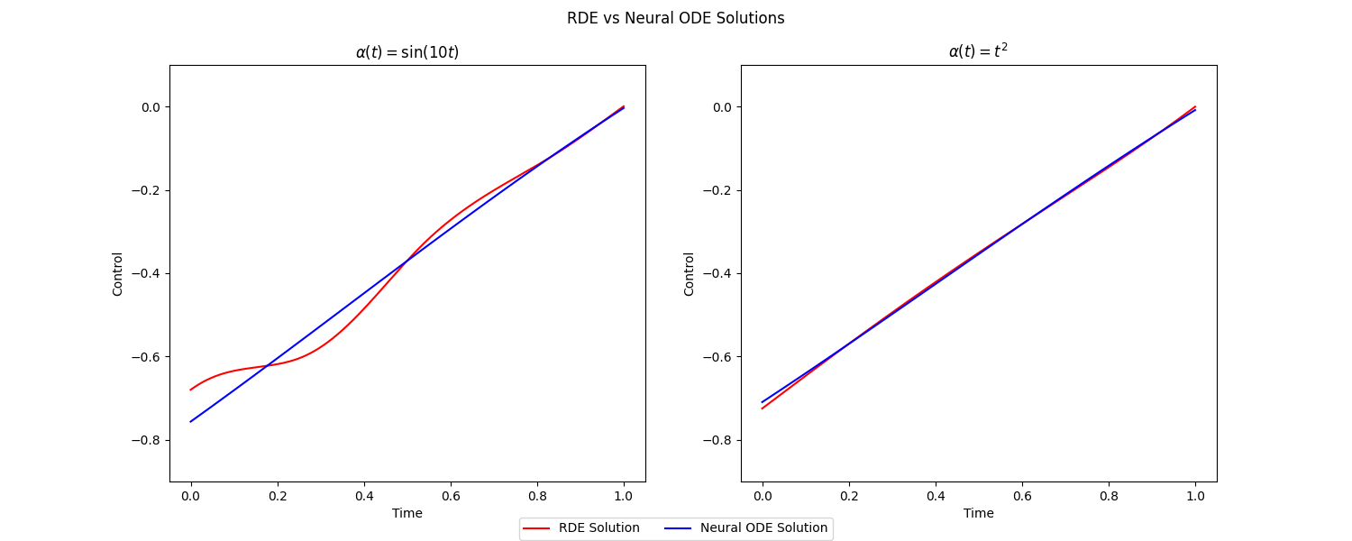
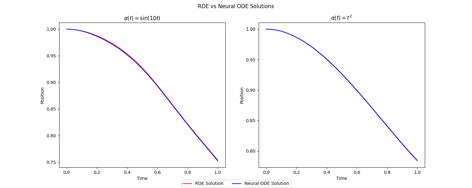
The control trajectories from the RDE and Neural ODE differ noticeably, although the resulting position trajectories remain similar. I hypothesized that the Neural ODE had reached a poor local optimum. To test this, I pretrained the MLP control $u_\theta$ to fit the RDE solution and then randomly perturbed the learned parameters before optimization.

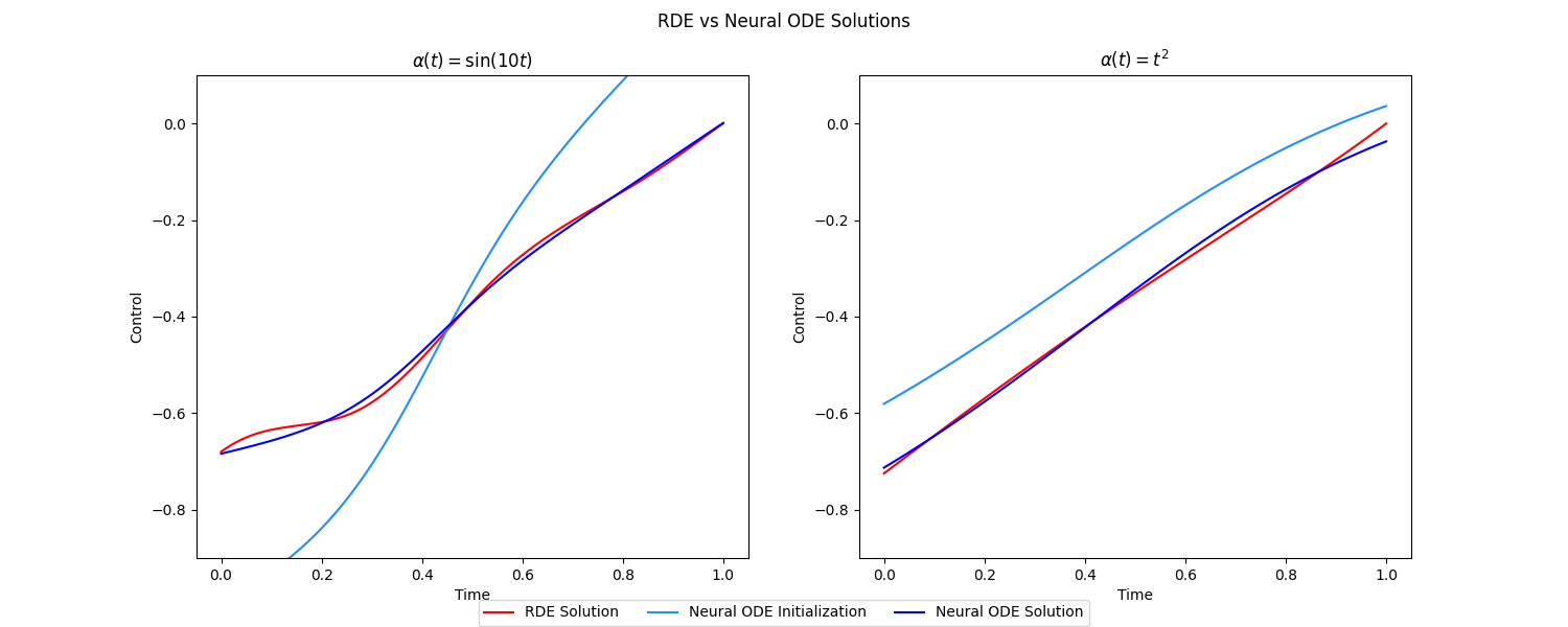
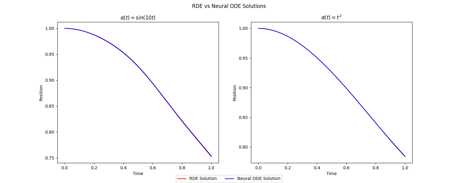
The solutions of the Neural ODE are indeed closer to those of the RDE method. Perhaps, if you zoom in very closely, the position trajectory from the Neural ODE solution is closer to the RDE solution (compared to the case without a learned initialization).

Some Discussions

In this simple example, the RDE solution is both more reliable and more efficient: it requires one forward and one backward pass through the numerical solver, whereas each of the 1000 Neural ODE optimization steps requires both. The Neural ODE applies to more general dynamics, while the Riccati method is restricted to structured problems such as LQR. The adjoint method can also use constant memory, whereas a directly discretized MSA must retain ${u(t^{(0)}),\ldots,u(t^{(n)})}$ across time steps.

We should notice that Neural ODE is essentially based on a relaxed version of the PMP, which does not necessarily guarantee optimality. This suggests that we may want to use better optimizers (e.g., momentum method or Nesterov accelerated gradient) or better initializations when applying Neural ODE to avoid sticking in local optima. For example, we may want to use a simple control trajectory that is sufficiently close to the optimal trajectory (albeit potentially non-optimal) to learn the initialization parameters, then use Neural ODE to fine-tune the result.

Additionally, physics-informed neural networks (PINNs) could be another deep learning approach for solving optimal control problems. In this framework, one can train a PINN to learn a value function that satisfies the HJB equation and subsequently extract the optimal control $u^\ast(\cdot)$. However, the term

may be intractable for automatic differentiation. One can instead learn a parameterized control $u_\theta$ that approximates $u^\ast$, and replace the infimum by

similar to the treatments in deep reinforcement learning.